3.2 — Marginal Productivity Theory
ECON 452 • History of Economic Thought • Fall 2022
Ryan Safner
Associate Professor of Economics
safner@hood.edu
ryansafner/thoughtF22
thoughtF22.classes.ryansafner.com
Second-Generation Marginalists

Primarily extended and applied Jevons, Menger, & Walras’ marginalist tendencies to more problems in economics
- especially, the problem of pricing the factors of production
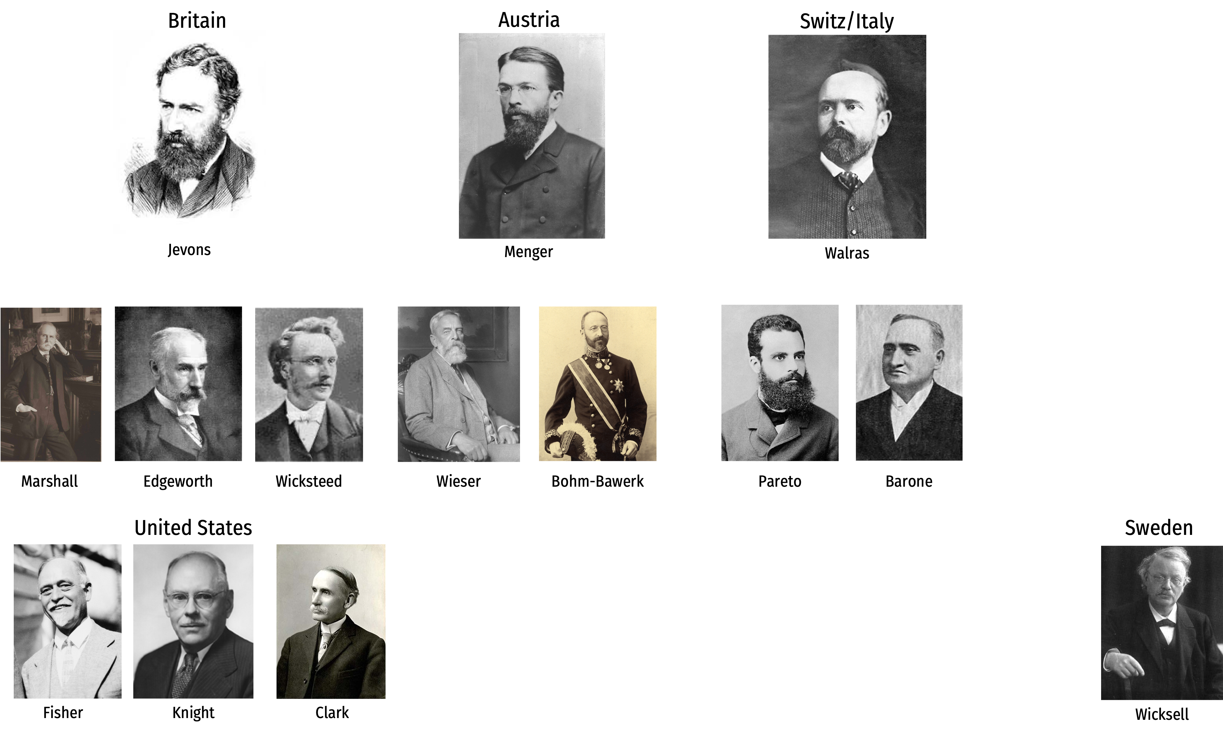
In England: Alfred Marshall, Phillip Wicksteed, Francis Edgeworth, A.C. Pigou
In Austria: Friedrich Wieser, Eugen von Böhm-Bawerk
In Switz./Italy: Enrico Barone, Vilfredo Pareto
In United States: John Bates Clark, Irving Fisher, Frank Knight, Frank Fetter, Frank Taussig
In Sweden: Knut Wicksell, Gustav Cassel
Second-Generation Marginalists
Second-Generation Austrian Marginalists
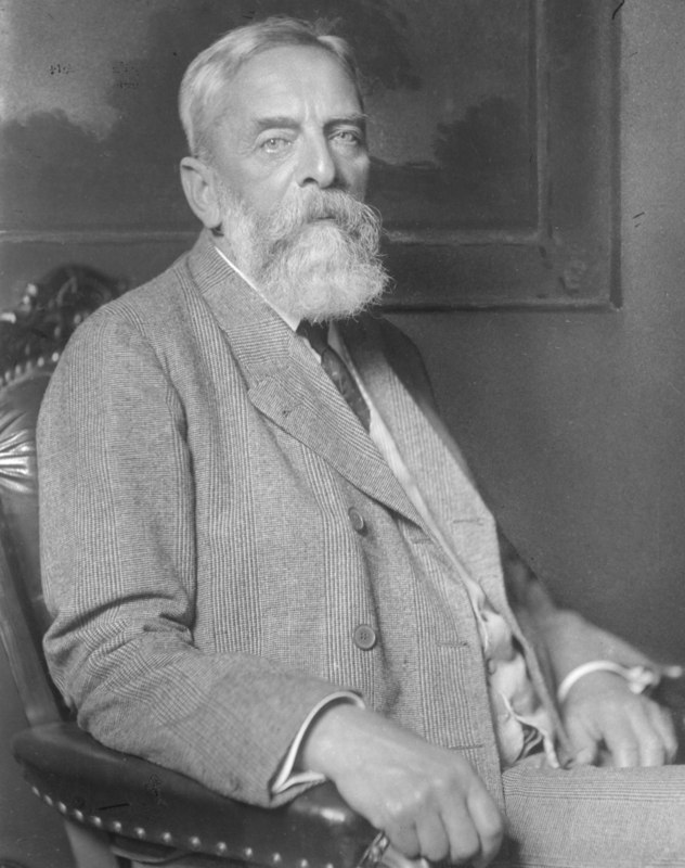
Friedrich von Wieser
Friedrich von Wieser
1851—1926
Student of Menger, ultimately replaced Menger as Professor of Political Economy at University of Vienna
Coined the term “marginal utility” (Grenznutzen)
Teacher to F.A. Hayek
1889, Der natürliche Werth (Natural Value)
1914, Theorie der gesellschaftlichen Wirtschaft (Theory of Social Economy),
Friedrich von Wieser: Alternative Cost Theory

Friedrich von Wieser
1851—1926
What role do costs of production (payments to factors) play in value of final goods?
Costs are the values which are forgone in directing resources to a particular production process rather than other production processes
In this sense, production costs are really a reflection of utilities elsewhere in the economy
Alternative cost theory or opportunity cost
Friedrich von Wieser: Alternative Cost Theory

Friedrich von Wieser
1851—1926
Beginnings of major disagreements:
Jevons always thought costs were “real” in some sense, e.g. the disutility or pain of labor
- utility of consumption vs. disutility of production; utility & disutility curves
Marshall & Edgeworth would later argue you can derive an upward-sloping supply/cost curve for non-land factors by disutility of use
Friedrich von Wieser: Imputation Theory

Friedrich von Wieser
1851—1926
Menger had clear insights about capital and production: goods of higher order, their complementarity and substitutability, etc.
If we all agree that prices of final goods reflect their marginal utility, how do we price factor services (land, labor, capital)?
Wieser, using a legal term, this is a “problem of imputation”
Friedrich von Wieser: Imputation Theory

Friedrich von Wieser
1851—1926
Wieser’s solution was linear programming with simultaneous equations (no calculus)
Example: consider a three-good society, factors in each good’s production are x, y, and z, represented by three simultaneous equations:
x+y=1002x+3z=2904y+5z=590
Solve for x, y, and z (prices of each factor)
Assumes prices for final goods are given, fixed production coefficients, and no substitution of factors
Wieser, Friedrich von, 1893, Natural Value p.88
Eugen von Böhm-Bawerk

Eugen von Böhm-Bawerk
1851—1914
Studied law at University of Vienna; exposed to Menger but never his direct student
Friend & brother-in-law to Friedrich Wieser
Became Minister of Finance of Austria-Hungary; amabassador to Germany
Later became professor of political economy, teacher to Ludwig von Mises
Eugen von Böhm-Bawerk

Eugen von Böhm-Bawerk
1851—1914
Direct critique of Marxism: 1896, Karl Marx and the Close of His System
Famously wrote on capital theory and interest theory
- We will dig into this next week
Capital & Interest 2 volumes:
- 1884, History and Critique of Interest Theories
- 1889, Positive Theory of Capital
Eugen von Böhm-Bawerk

Eugen von Böhm-Bawerk
1851—1914
Took a different approach to the imputation problem (factor pricing) than Wieser:
Followed a phrase in Menger, “the loss principle” — applying to the price of the final good what would be lost if one of the factor services is withdrawn
A good start, but in truth, marginal product operates at infinitesimally small changes (derivative)
Eugen von Böhm-Bawerk: On Opportunity Cost

Eugen von Böhm-Bawerk
1851—1914
“If in any branch of production the price sinks below the cost...men will withdraw from that branch and engage in some better paying branch of production. Conversely, if in one branch of production, the market price of the finished good is considerably higher than the value of the sacrificed or expended means of production, then will men be drawn from less profitable industries. They will press into the better paying branch of production, until through the increased supply, the price is again forced down to cost.
Böhm-Bawerk, Eugen von, 1884, Capital and Interest
Eugen von Böhm-Bawerk: On Opportunity Cost

Eugen von Böhm-Bawerk
1851—1914
“What determine the amount of this cost? The amount of the cost is identical with the value of the productive power, and, as a rule, is determined by the money marginal utility of this productive power...The price of a definite specie of freely reproducible goods fixes itself in the long run at that point where the money marginal utility, for those who desire to purchase these products, intersects the money marginal utility of all those who desire to purchase in the other communicating branches of production. The figure of the two blade of a pair of shears still holds good. One of the two blade, whose coming together determine the height of the price of any species of product, is in truth the marginal utility of this particular product. The other, which we are wont to call "cost," is the marginal utility of the products of other communicating branches of production. Or, according to Wieser, the marginal utility of "production related goods." It is, therefore, utility and not disutility which, as well on the side of supply as of demand, determine the height of the price. This, too, even where the so-called law of cost plays its role in giving value to goods. Jevons, therefore, did not exaggerate the importance of the one side, but came very near the truth when he said "value depends entirely upon utility.” (45)
Price is Determined at the Margin: B-B’s Example

Imagine a small public horse market
3 people, A, B, and C each own 1 horse
3 people, D, E, and F each are potentially interested in buying a horse
This example is based on Eugen von Bohm-Bawerk’s famous example in Capital and Interest (1884)
Price is Determined at the Margin: B-B’s Example
| Person | Reservation Price |
|---|---|
| A | Minimum WTA: $400 |
| B | Minimum WTA: $500 |
| C | Minimum WTA: $600 |
| D | Maximum WTP: $600 |
| E | Maximum WTP: $500 |
| F | Maximum WTP: $400 |
Imagine a small public horse market
3 people, A, B, and C each own 1 horse
3 people, D, E, and F each are potentially interested in buying a horse
Price is Determined at the Margin: B-B’s Example
| Person | Reservation Price |
|---|---|
| A | Minimum WTA: $400 |
| B | Minimum WTA: $500 |
| C | Minimum WTA: $600 |
| D | Maximum WTP: $600 |
| E | Maximum WTP: $500 |
| F | Maximum WTP: $400 |
Price: $400
Suppose Buyer F announces she will pay $400 for a horse
Only Seller A is willing to sell at $400
Buyers D, E, and F are willing to buy at $400
- D and E are willing to pay more than F to obtain the 1 horse
- A shortage: 3 buyers for 1 seller!
- They raise their bids above $400 to attract sellers
Price is Determined at the Margin: B-B’s Example
| Person | Reservation Price |
|---|---|
| A | Minimum WTA: $400 |
| B | Minimum WTA: $500 |
| C | Minimum WTA: $600 |
| D | Maximum WTP: $600 |
| E | Maximum WTP: $500 |
| F | Maximum WTP: $400 |
Price: $600
Suppose Seller C announces he will sell his horse for $600
Only Buyer D is willing to buy at $600
Sellers A, B, and C are willing to sell at $600
- A and B are willing to accept less than C to sell their horses
- A surplus: 3 sellers for 1 buyer!
- They lower their asks below $600 to attract buyers
Price is Determined at the Margin: B-B’s Example
| Person | Reservation Price |
|---|---|
| A | Minimum WTA: $400 |
| B | Minimum WTA: $500 |
| C | Minimum WTA: $600 |
| D | Maximum WTP: $600 |
| E | Maximum WTP: $500 |
| F | Maximum WTP: $400 |
Price: $500
If the market price reaches $500 (through bids and asks changing):
Sellers A and B sell their horses for $500 each
- Buyers D and E buy them at $500 each
Price is Determined at the Margin: B-B’s Example
| Person | Reservation Price |
|---|---|
| A | Minimum WTA: $400 |
| B | Minimum WTA: $500 |
| C | Minimum WTA: $600 |
| D | Maximum WTP: $600 |
| E | Maximum WTP: $500 |
| F | Maximum WTP: $400 |
Price: $500
At $500, B and E are the “marginal” buyer and seller, the “last” ones that just got off the fence to exchange in the market
- B has WTA just low enough to sell
- E has WTP just high enough to buy
The marginal pair actually are the ones that “set” the market price!
Price is Determined at the Margin: B-B’s Example
| Person | Reservation Price |
|---|---|
| A | Minimum WTA: $400 |
| B | Minimum WTA: $500 |
| C | Minimum WTA: $600 |
| D | Maximum WTP: $600 |
| E | Maximum WTP: $500 |
| F | Maximum WTP: $400 |
Price: $500
Notice the most possible exchanges take place at a market price of $500
- 2 horses get exchanged
Any price above or below $500, only 1 horse would get exchanged
- Also, at least one other buyer or seller would raise/lower their bid/ask
Price is Determined at the Margin: B-B’s Example
| Person | Reservation Price |
|---|---|
| A | Minimum WTA: $400 |
| B | Minimum WTA: $500 |
| C | Minimum WTA: $600 |
| D | Maximum WTP: $600 |
| E | Maximum WTP: $500 |
| F | Maximum WTP: $400 |
Price: $500
- At $500, C and F are the "excluded" buyers and sellers
- C has WTA too high to sell
- F has WTP too low to buy
Price is Determined at the Margin: B-B’s Example
| Person | Reservation Price |
|---|---|
| A | Minimum WTA: $400 |
| B | Minimum WTA: $500 |
| C | Minimum WTA: $600 |
| D | Maximum WTP: $600 |
| E | Maximum WTP: $500 |
| F | Maximum WTP: $400 |
Price: $500
At $500, A and D are the "inframarginal" buyers and sellers
- A has WTA lower than market price, earns extra $100 surplus from exchange
- D has WTP higher than market price, earns extra $100 surplus from exchange
These buyers and sellers benefit the most from exchange
Marginal Productivity Theory
The Ricardian Roots of Marginal Productivity Theory

David Ricardo
1772-1823
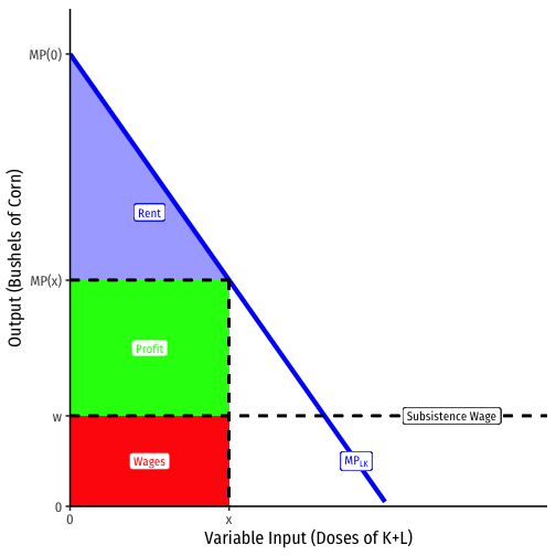
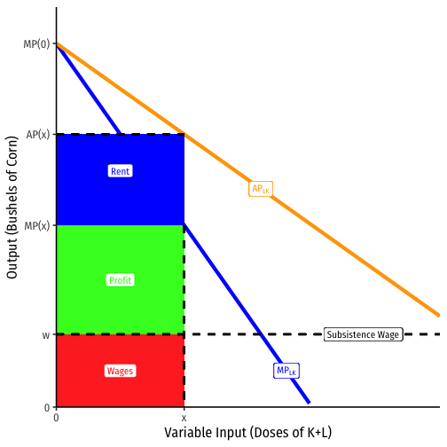
Ricardo’s theory of rent applied marginal analysis (“doses” of L+K) to a fixed factor (land), concluding the fixed factor earns a residual surplus (gap between AP>MP) of variable factor (L+K)
Marginal productivity theory both generalizes and repudaites Ricardian approach: any variable factor must earn a payment equal to its marginal product (holding all other factors fixed)
- i.e. nothing special about land — get the same results if it’s capital or labor that’s held fixed!
Marginal Productivity Theory
Applying Ricardian logic beyond agriculture, we arrive at the modern law of diminishing returns
- “Law of variable proportions” or “variation of returns”
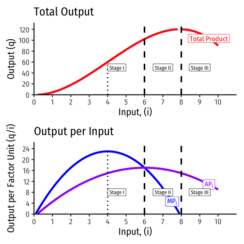
For any one variable factor (holding all others constant), increasing use will eventually yield a diminishing marginal product
Diminishing Returns
Marginal product of factor i, (MPi): additional output produced by adding one more unit of factor i (holding all others constant) MPi=ΔqΔi
- MPi is slope of TP at each value of i
Average product of factor i (APi): additional output produced by adding one more unit of factor i (holding all others constant) APi=qi
- APi is slope of a ray from the origin to the production function at any quantity of i

Derived Demand in Factor Markets
Demand for factors (e.g. labor) is a “derived demand”:
- Firm only demands inputs to the extent they contribute to producing sellable output
Firm faces a tradeoff when hiring more labor, as more labor ΔL creates:
- Marginal Benefit: Increases output and thus revenue
- Marginal Cost: Increases costs

Marginal Revenue Product (of Labor)
- Hiring more labor increases output (i.e. labor's MPL)
- Recall: MPL=ΔqΔL, where q is units of output
Marginal Revenue Product (of Labor)
Hiring more labor increases output (i.e. labor's MPL)
- Recall: MPL=ΔqΔL, where q is units of output
Additional output generates (i.e. labor's MR(q))
- Recall: MR(q)=ΔR(q)Δq, where R(q) is total revenue
Marginal Revenue Product (of Labor)
Hiring more labor increases output (i.e. labor's MPL)
- Recall: MPL=ΔqΔL, where q is units of output
Additional output generates (i.e. labor's MR(q))
- Recall: MR(q)=ΔR(q)Δq, where R(q) is total revenue
- Hiring more labor, on the margin, generates a benefit, called the marginal revenue product of labor, MRPL:
MRPL=MPL∗MR(q)
- i.e. the number of new products a new worker makes times the revenue earned by selling the new products
Marginal Revenue Product for Competitive Firms
- This is the Firm's Demand for Labor:
MRPL=MPL∗MR(q)
- For a firm in a competitive (output) market, firm's MR(q)=p, hence:
MRPL=MPL∗p where p is the price of the firm's output

Marginal Revenue Product for Competitive Firms
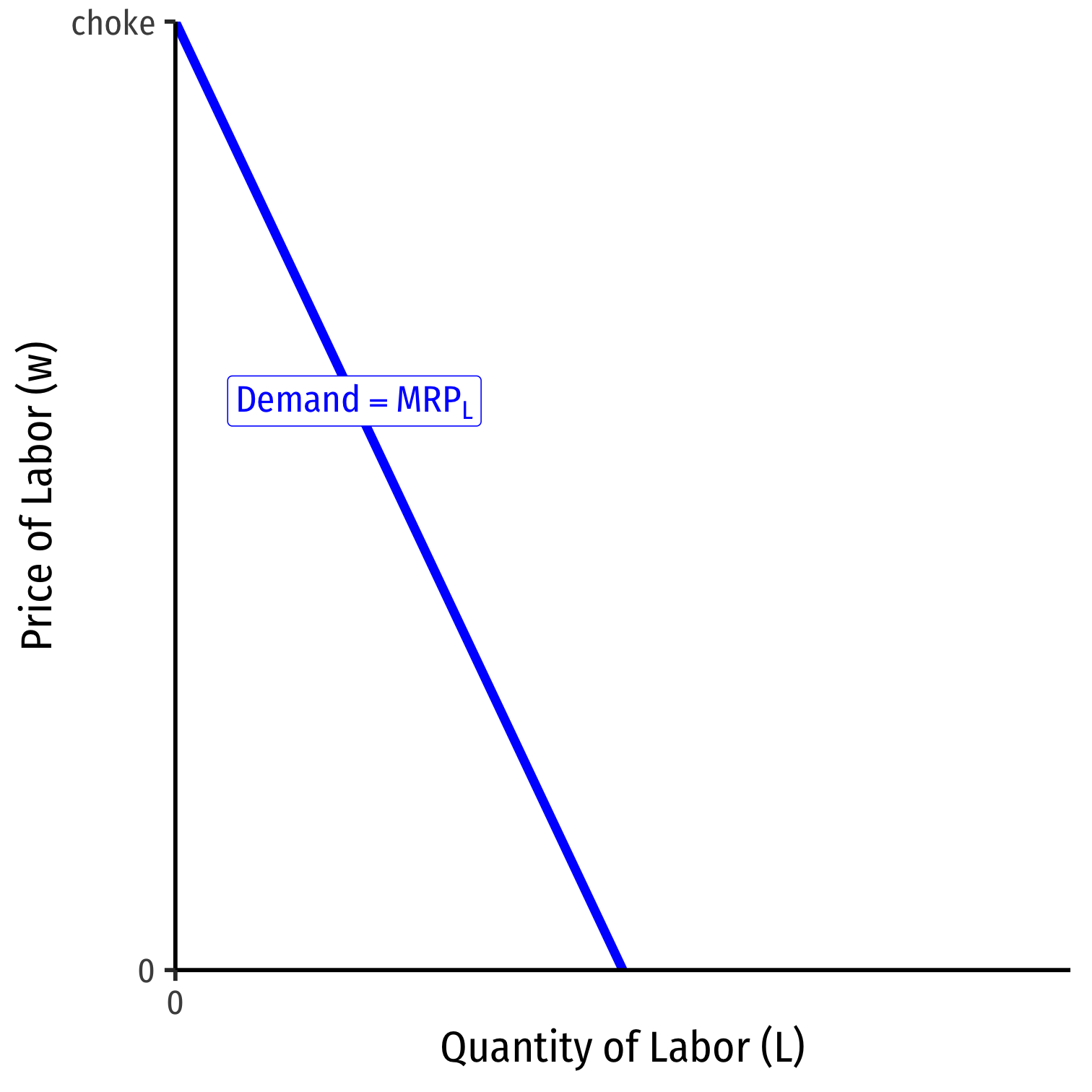
MRPL=MPL∗p
Marginal benefit of hiring labor, MRPL falls with more labor used
- production exhibits diminishing marginal returns to labor!
Choke price for labor demand: price too high for firm to purchase any labor
A Competitive Factor Market
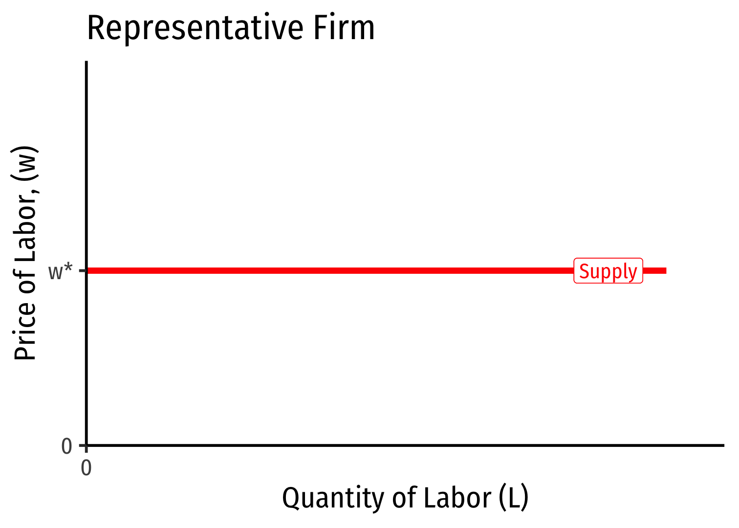
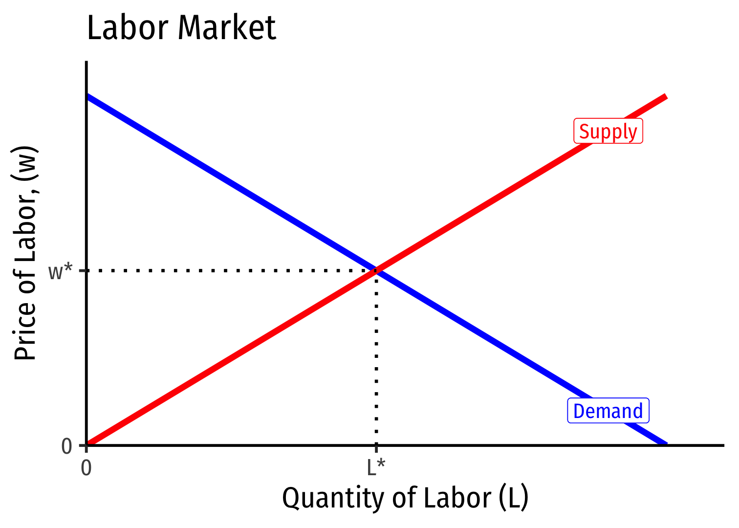
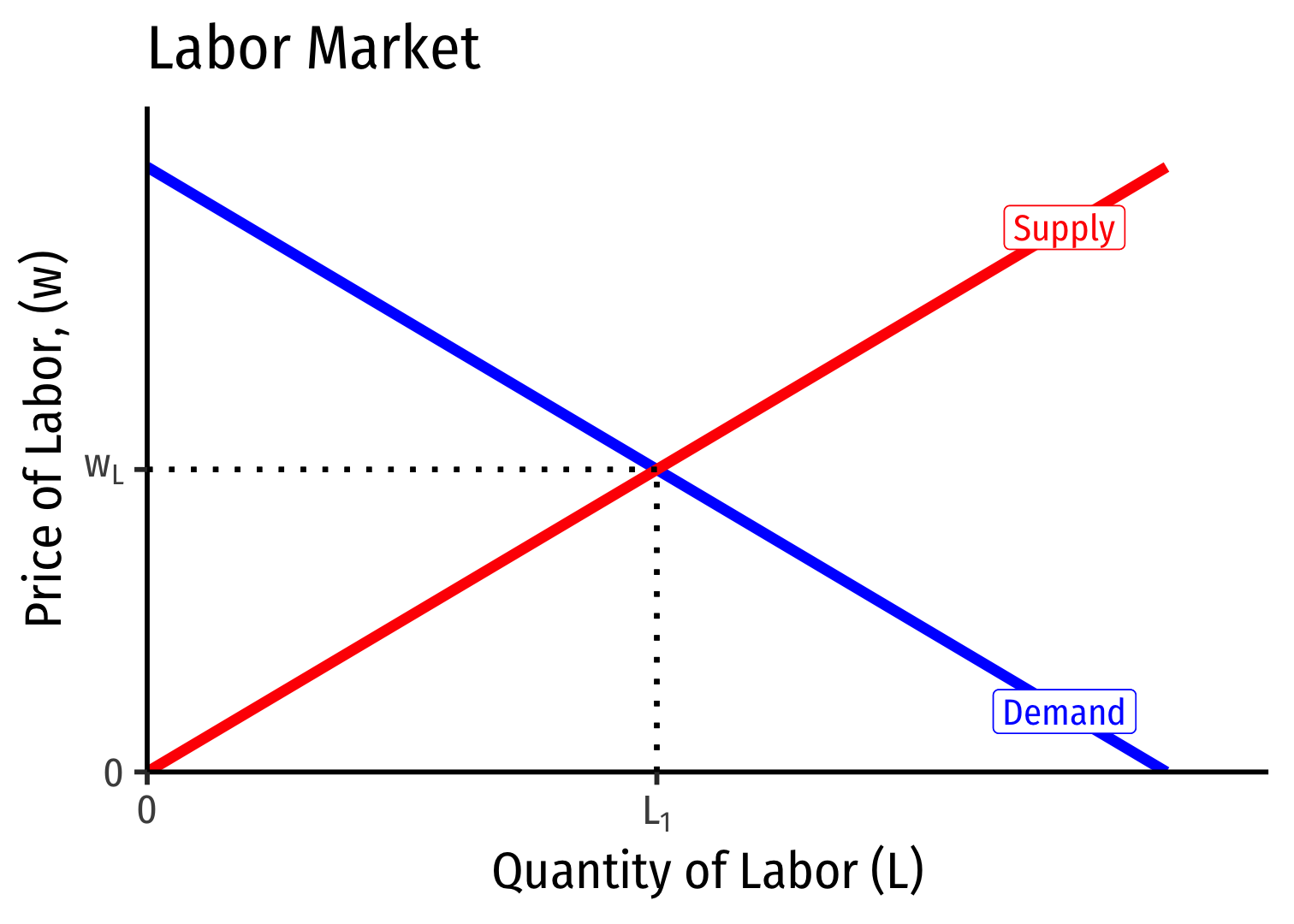
- If the factor market is competitive, labor supply for an individual firm is perfectly elastic at the market price of labor (w∗)
Labor Supply and Firm's Demand for Labor
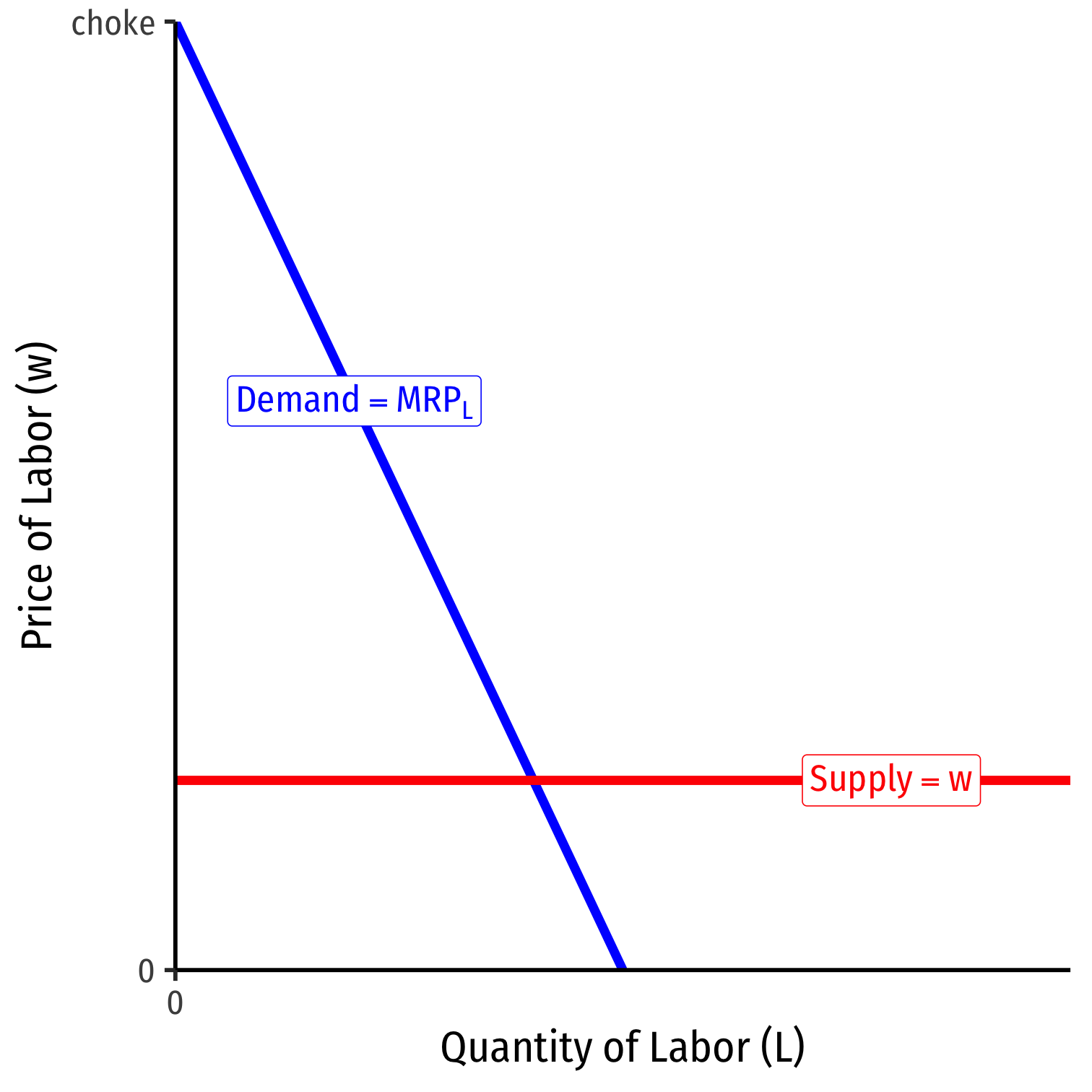
We've seen a falling MRPL, the marginal benefit of hiring labor
Marginal cost of hiring labor, w, remains constant
- so long as firm is not a big purchaser (has no market power) in the labor market
Labor Supply and Firm's Demand for Labor
At low amounts of labor, marginal benefit (MRPL)>w marginal cost
Firm will hire more labor
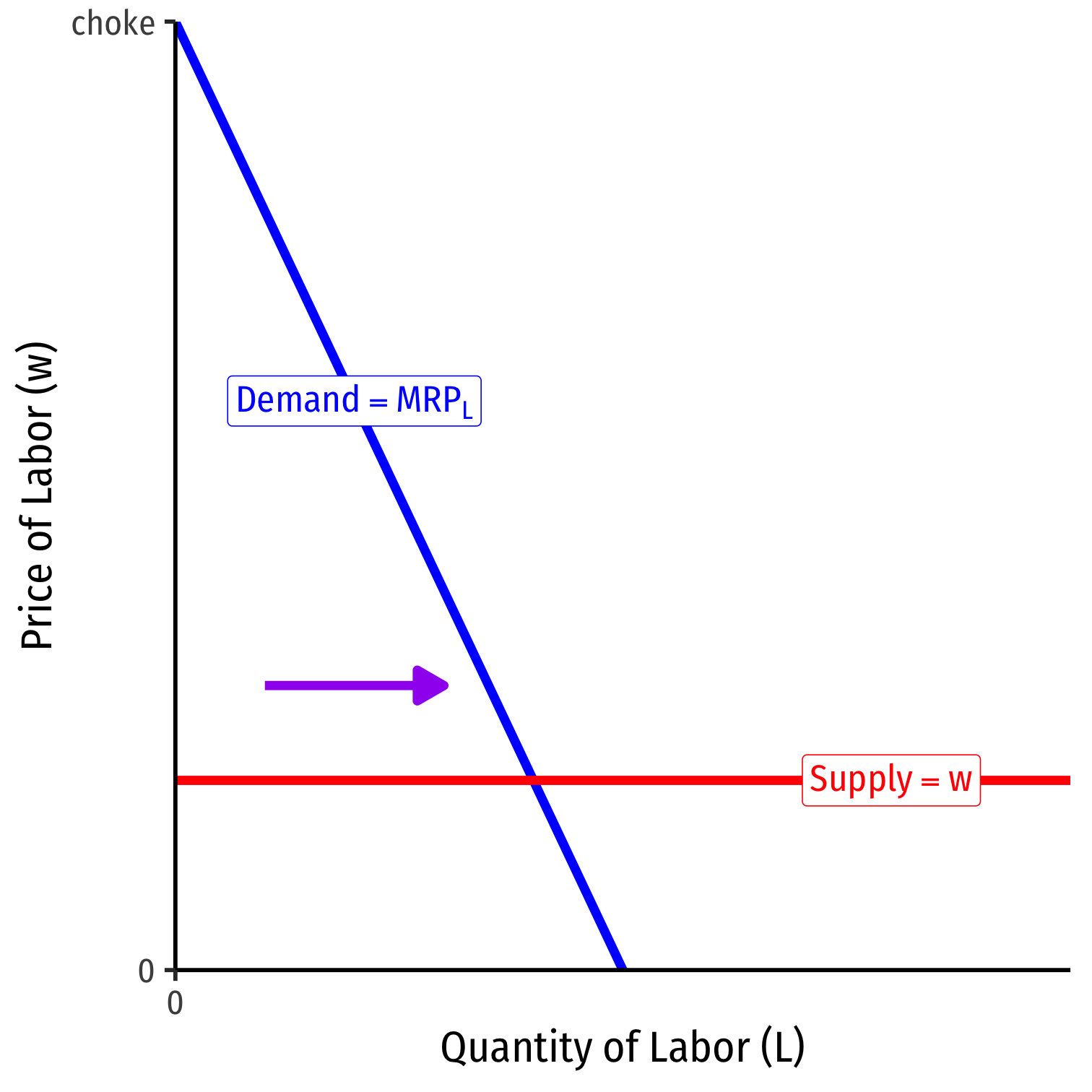
Labor Supply and Firm's Demand for Labor
At high amounts of labor, marginal benefit (MRPL)<w marginal cost
Firm will hire less labor
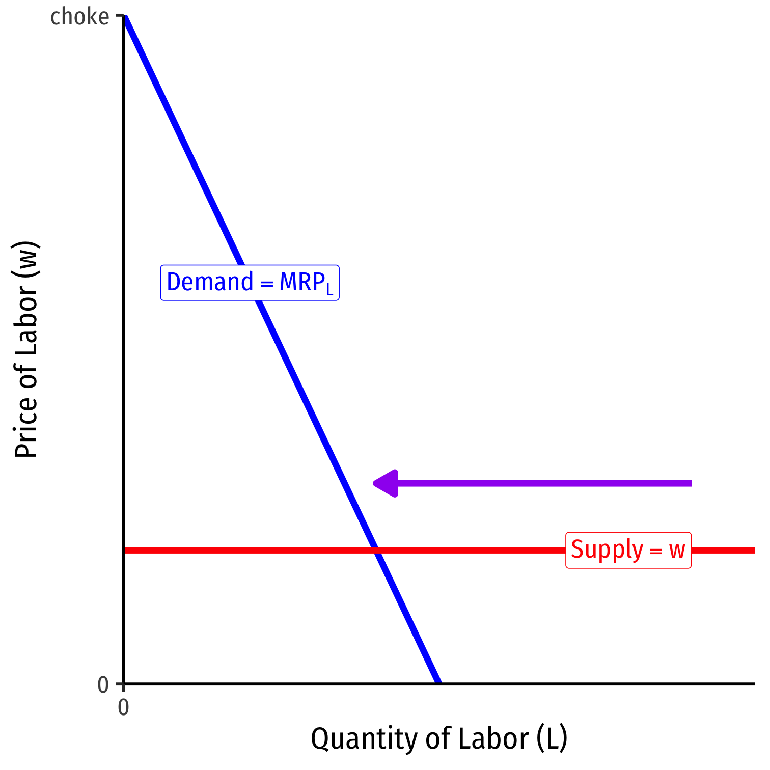
Labor Supply and Firm's Demand for Labor
Firm hires L∗ optimal amount of labor where w=MRPL
i.e. marginal cost of labor = marginal benefit of labor
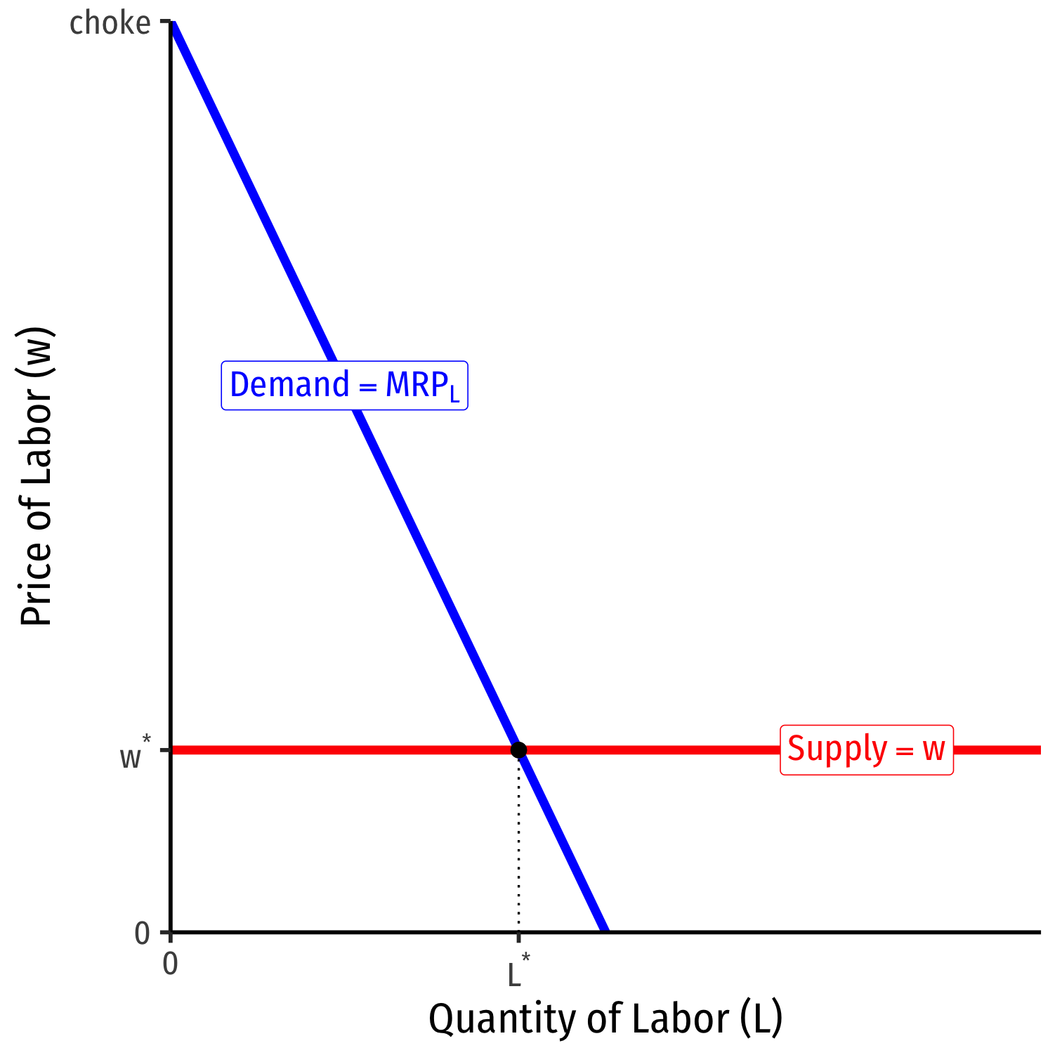
Labor Supply and Firm's Demand for Labor
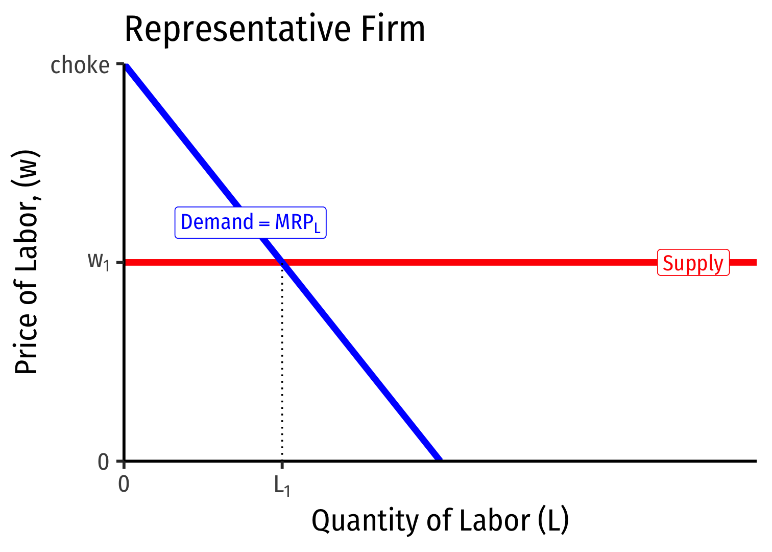
Labor Supply and Firm's Demand for Labor
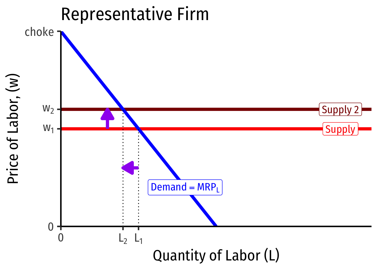
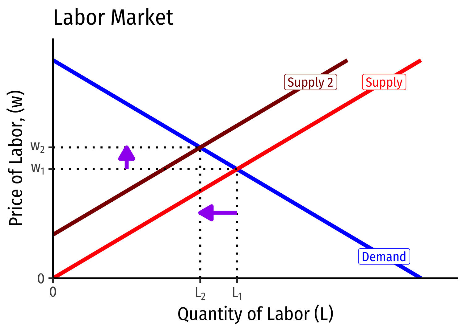
- If market supply of labor decreases, firms hire fewer workers, at higher wages (and vice versa)
Multiple Inputs and Cost Minimization
But firms produce with many factors, what is the more general rule for hiring the optimal combination of factors?
Assume three factors: land, labor, capital
Optimal hiring condition is the equimarginal rule (Gossen’s Second Law} again:
MPlpl=MPkpk=MPtpt=⋯=MPnpn
- Cost of production is minimized where the marginal product per dollar spent is equalized across all n possible inputs
- the “last dollar spent” on each input provides the same marginal product

The Product Exhaustion Debates & Marginal Productivity Theory
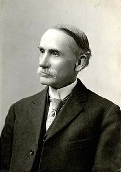
John Bates Clark
John Bates Clark
1847—1938
Initially a German Historicist (studied under Karl Knies) in Germany; a Christian socialist
Became professor at Columbia, independently derived his own version of marginal utility theory
First to formulate & popularize marginal productivity theory, virtues of market competition; opponent to American Institutionalists (see later)
1886, The Philosophy of Wealth
1889, “Possibility of a Scientific Law of Wages” paper at AEA; generalized in 1899 The Distribution of Wealth
The Product Exhaustion Debate
Ricardian rent theory defined rent as a residual, will always adjust to fill the gap between output price and wages & profits
- output price = wages & profits + rent
Thus, the payments to all factors of production (land, labor, capital) “fully exhaust the product”
- i.e. the sum of factor payments (costs to firm) equals the price
Product Exhaustion Debate
- In competitive markets, each factor is paid its marginal (revenue) product (shown above)
Product Exhaustion Debate
In competitive markets, each factor is paid its marginal (revenue) product (shown above)
Product exhaustion debate: does the sum of these marginal products exactly equal the market price of the output?
Product Exhaustion Debate
In competitive markets, each factor is paid its marginal (revenue) product (shown above)
Product exhaustion debate: does the sum of these marginal products exactly equal the market price of the output?
Q=?MPLL+MPKK+MPTT
Product Exhaustion Debate
In competitive markets, each factor is paid its marginal (revenue) product (shown above)
Product exhaustion debate: does the sum of these marginal products exactly equal the market price of the output?
Q=?MPLL+MPKK+MPTT pQ=?(P∗MPL)L+(p∗MPK)K+(p∗MPT)T
Product Exhaustion Debate
In competitive markets, each factor is paid its marginal (revenue) product (shown above)
Product exhaustion debate: does the sum of these marginal products exactly equal the market price of the output?
Q=?MPLL+MPKK+MPTT pQ=?(P∗MPL)L+(p∗MPK)K+(p∗MPT)T pQ=?(MRPL)L+(MRPK)K+(MRPT)T
- The claim that it does is the essence of marginal productivity theory
John Bates Clark: Marginal Productivity Theory

John Bates Clark
1847—1938
- Clark famously argued that on a competitive market, each factor is paid its marginal product, and that this exactly exhausts the product
Q=MPL×L+MPK×K+MPT×T
- Offered little proof that this is true
Phillip Wicksteed
Phillip Wicksteed
1844—1927
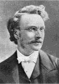
A British economist and unitarian minister
Learned economics from Jevons, and got inspired to write about political economy after reading Henry George
1894, An Essay on the Co-Ordination of the Laws of Distribution
- tries to solve the product exhaustion problem of marginal productivity theory
1910, The Common Sense of Political Economy: Including a Study of the Human Basis of Economic Law
- one of the greatest books popularizing marginalism
Proving Product Exhaustion...Sort Of

Phillip Wicksteed
1844—1927
- Uses Euler’s Theorem of homogeneous functions to prove product exhaustion under specific conditions:
- production functions must be linearly homogenous (of degree 1)
cnY=f(cnL,cnK,cnT):n=1
- we would say: “constant returns to scale”
- Heavily criticized for this!
Returns to Scale
- The returns to scale of production: change in output when all inputs are increased at the same rate (scale)

Returns to Scale
The returns to scale of production: change in output when all inputs are increased at the same rate (scale)
Constant returns to scale: output increases at same proportionate rate to inputs change
- e.g. double all inputs, output doubles

Returns to Scale
The returns to scale of production: change in output when all inputs are increased at the same rate (scale)
Constant returns to scale: output increases at same proportionate rate to inputs change
- e.g. double all inputs, output doubles
Increasing returns to scale: output increases more than proportionately to inputs change
- e.g. double all inputs, output more than doubles

Returns to Scale
The returns to scale of production: change in output when all inputs are increased at the same rate (scale)
Constant returns to scale: output increases at same proportionate rate to inputs change
- e.g. double all inputs, output doubles
Increasing returns to scale: output increases more than proportionately to inputs change†
- e.g. double all inputs, output more than doubles
Decreasing returns to scale: output increases less than proportionately to inputs change
- e.g. double all inputs, output less than doubles

† See my new newsletter Increasing Returns for more on the importance of this idea
Constant Returns to Scale
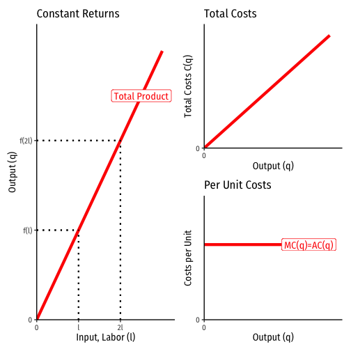
Constant returns to scale: doubling all inputs ⟹ double output f(cl,ck,ct)=cf(l,k,t)∀c>1
Constant economies of scale: average and marginal costs (are equal and) do not vary with output
Total revenues are completely exhausted by the payments to factors (costs to firm)
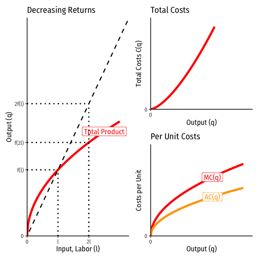
Decreasing Returns to Scale
Decreasing returns to scale: doubling all inputs ⟹ less than double output f(cl,ck,ct)<cf(l,k,t)∀c>1
Diseconomies of scale: average and marginal costs are increasing with output
- AC < MC ⟹ marginal cost pricing is always profitable
- Total Costs < Total Revenues ⟹π>0
Total revenues are not exhausted by the payments to factors (costs to firm); residual profits leftover!
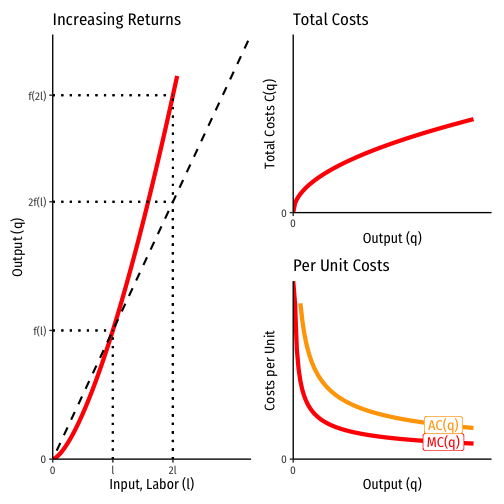
Increasing Returns to Scale
Increasing returns to scale: doubling all inputs ⟹ more than double output f(cl,ck,ct)>cf(l,k,t)∀c>1
Economies of scale: average and marginal costs are decreasing with output
- AC > MC ⟹ marginal cost pricing is always loss-inducing
- Total Costs > Total Revenues ⟹π<0
Total revenues are insufficient to cover the payments to factors (costs to firm); losses!
Criticisms of Wicksteed
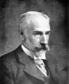
Francis Ysidro Edgeworth
1845-1926
“This is certainly a remarkable discovery; for the relation between product and factors is to be considered to hold good irrespectively of the play of the market...There is a magnificence in this generalization which recalls the youth of philosophy. Justice is a perfect cube, said the ancient sage; and rational conduct is a homogeneous function, adds the modern savant.”
Edgeworth, Francis Ysidro, 1904, "The Theory of Distribution," Quarterly Journal of Economics 18, p.149-219.
Criticisms of Wicksteed

Sir John Hicks
1904-1989
Economics Nobel 1972
“Where Wicksteed went wrong was his assumption that he could argue from the shape of the curve at one particular point to the general shape of the curve.”
Edgeworth, Francis Ysidro, 1904, "The Theory of Distribution," Quarterly Journal of Economics 18, p.149-219.
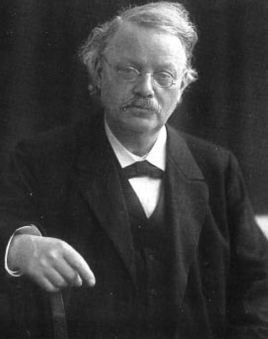
Knut Wicksell
Knut Wicksell
1851—1926
Swedish economist at University of Stockholm
Another supposed independent discoverer of marginal productivity theory
Made key contributions to capital and interest theory, influence Austrian & Keynesian schools of macroeconomics
- (we'll explore more next class)
1898, Interest and Prices
Wicksell and Product Exhaustion

Knut Wicksell
1851—1926
Most economists believed that an industry would always be either constant, increasing, or decreasing returns
Wicksell showed that most firms actually go through all three phases of returns to scale
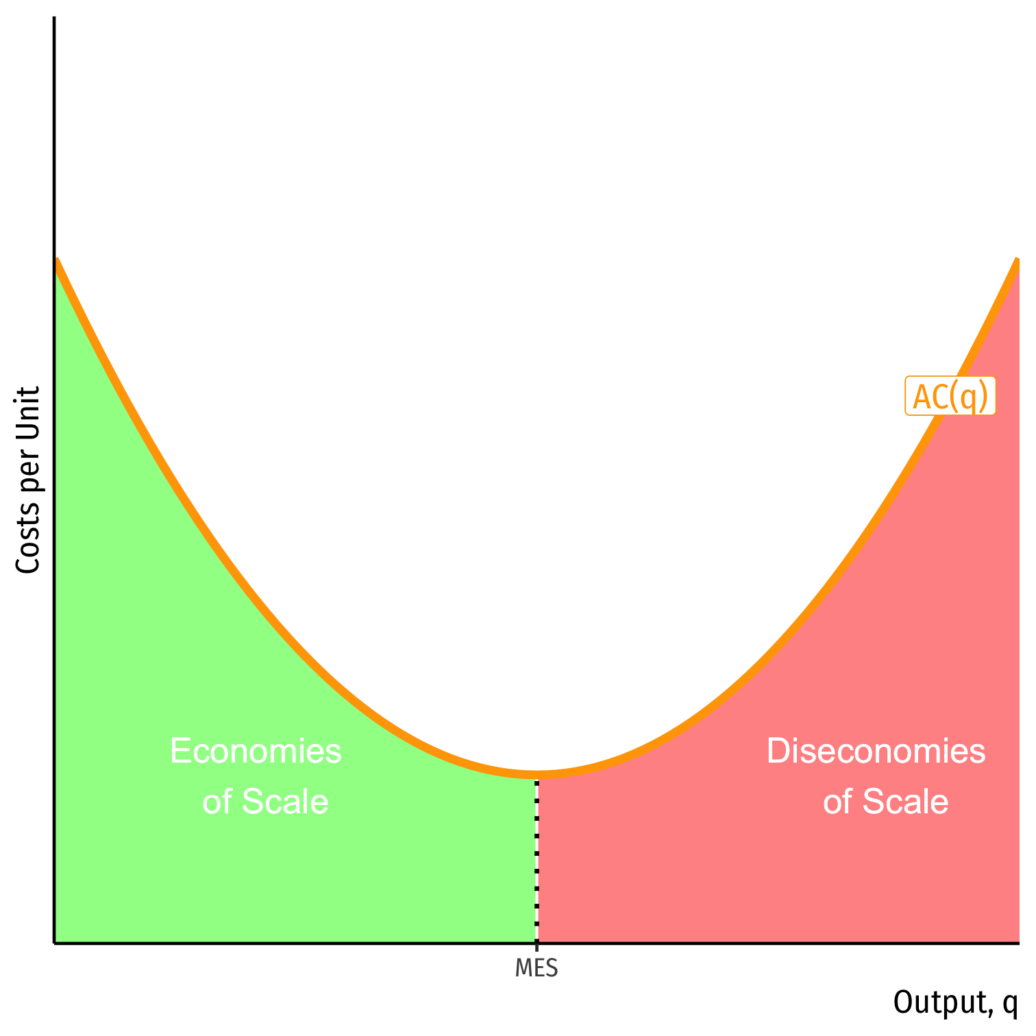
- developing a long-run U-shaped average cost curve for a firm
- would take a few decades for neoclassical economists to derive and understand shape of AC curve
Wicksell and Product Exhaustion

Knut Wicksell
1851—1926
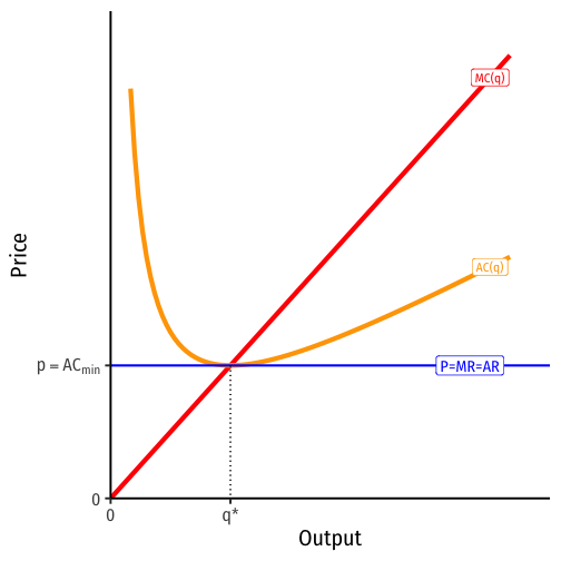
Thus, it is not necessary (as Wicksteed did) to assume constant returns to prove product exhaustion
Competition would ensure that in the long run, firms are producing at their least-cost combination
- p=MC=ACmin
- π=0
- “product exhaustion”
Long Run Costs & Scale Economies
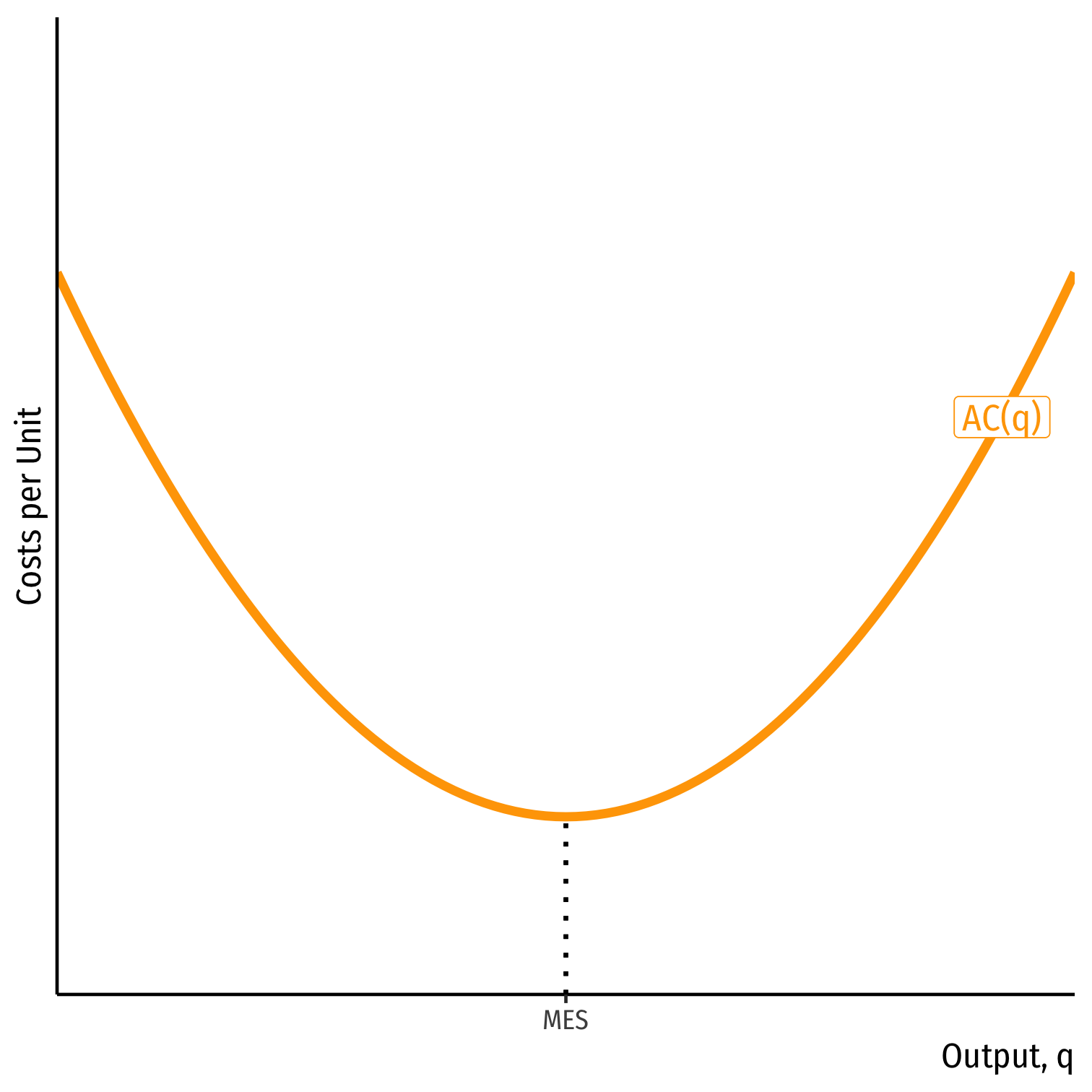
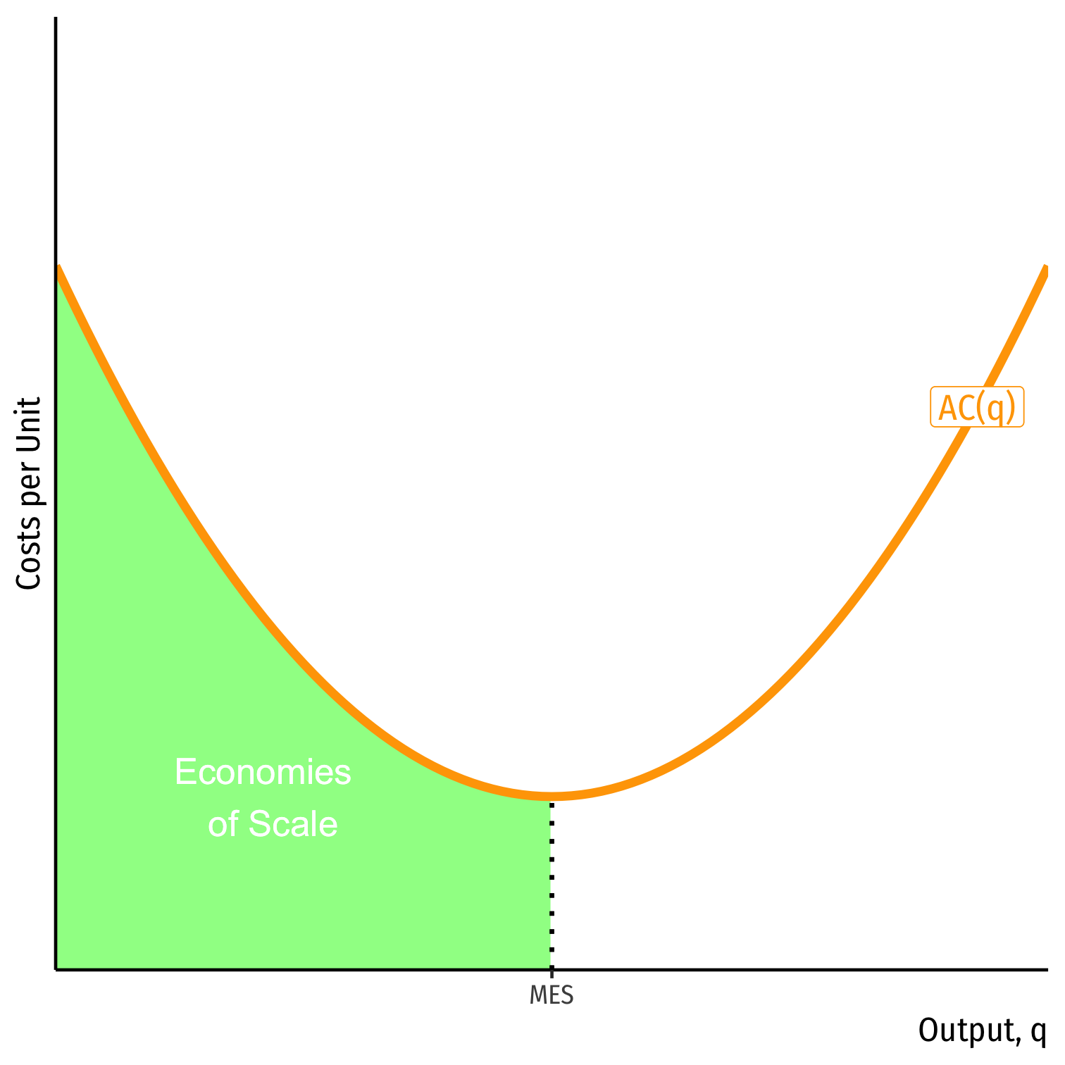
- Minimum Efficient Scale: q with the lowest AC(q)
- “optimal firm size”
Long Run Costs & Scale Economies
Minimum Efficient Scale: q with the lowest AC(q)
- “optimal firm size”
Economies of Scale: ↑q, ↓AC(q)
Long Run Costs & Scale Economies
Minimum Efficient Scale: q with the lowest AC(q)
- “optimal firm size”
Economies of Scale: ↑q, ↓AC(q)
Diseconomies of Scale: ↑q, ↑AC(q)
Wicksell and Product Exhaustion
Think about what you learn in microeconomics
In the long run, as profits attract entrants and losses force exits, price settles on the break-even point, where profit is 0
- p=MC=ACmin
- factors are paid their opportunity costs (marginal products); nothing leftover
We are gearing towards the origins of the perfect competition model
Implications & Criticisms of Marginal Productivity Theory
Implications of Marginal Productivity Theory

John Bates Clark
1847—1938
Several flaws with marginal productivity theory as a theory of distribution
MPT is primarily a theory of factor pricing, not about distribution of relative shares
It’s even an incomplete theory of factor pricing!
- Considers only demand side of factor market (firms), not the supply side!
Assumes competitive output and input markets
- Labor unions, monopsony power, bargaining, etc.
Implications of Marginal Productivity Theory
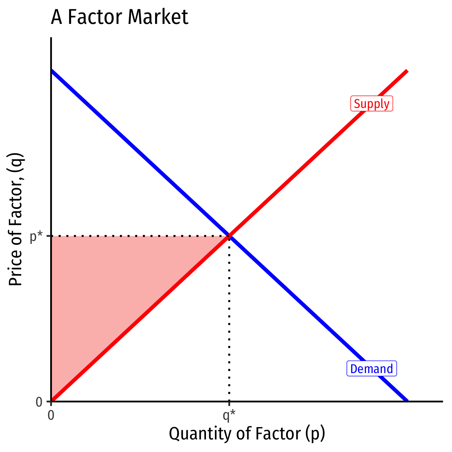
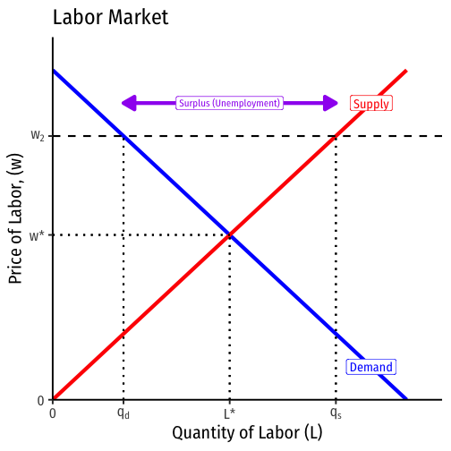
Factor employment is determined by supply & demand of factor, where demand is driven by the factor’s marginal revenue product
- if market price is above equilibrium (e.g. w2), a surplus (unemployment) of that factor
Prices will adjust downwards to equilibrium
Implications of Marginal Productivity Theory
What implications does this have for macroeconomic policy?
Applied to the entire economy, implies that (non-frictional) unemployment is due to above-equilibrium factor prices
- markets will correct this by adjusting prices downwards
Anticipating Keynes:
- but is it that easy to lower wages??
- if workers have less income, will that affect aggregate demand?

Implications of Marginal Productivity Theory

John Bates Clark
1847—1938
MPT describes the outcome to which we are always approaching (i.e. perfect competition), it is an equilibrium state of rest
- actual prices in real world are not equilibrium prices, we are not in perfect competition
In long run equilibrium in perfect competition, factor prices are paid their marginal products
- p=MC, all factors are paid opportunity costs, firms break even and “exhaust the product” AR(q)=AC(q)
Misconceptions About Marginal Productivity Theory
- Mistaken interpretation that MPT says factor prices are determined by their marginal products
- i.e. wage is determined by MPL
- A lot of Clark’s tone seems to imply this
Misconceptions About Marginal Productivity Theory
- Mistaken interpretation that MPT says factor prices are determined by their marginal products
- i.e. wage is determined by MPL
- A lot of Clark’s tone seems to imply this
- In truth, MPT says the opposite!: the quantity of factors employed (and thus their MP's) depends on factor prices!
- Factor prices are determined by supply & demand, period.
Misconceptions About Marginal Productivity Theory
- Mistaken interpretation that MPT says factor prices are determined by their marginal products
- i.e. wage is determined by MPL
- A lot of Clark’s tone seems to imply this
In truth, MPT says the opposite!: the quantity of factors employed (and thus their MP's) depends on factor prices!
- Factor prices are determined by supply & demand, period.
MPT is a description of factor markets in equilibrium: factors are paid their marginal products
- In essence, factor payments are a measure of MP in equilibrium
Misconceptions About Marginal Productivity Theory
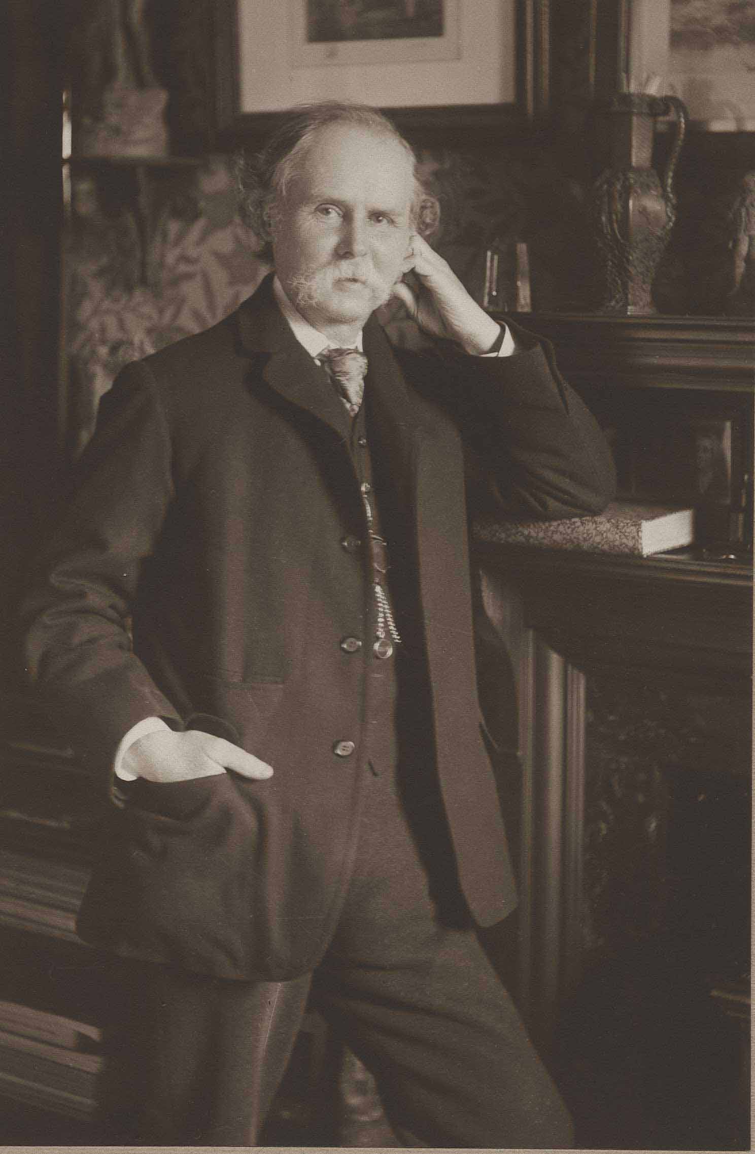
Alfred Marshall
1842-1924
“This [marginal productivity] doctrine has sometimes been put forward as a theory of wages. But there is no valid ground for any such pretension. The doctrine that the earnings of a worker tend to be equal to the net product of his work, has by itself no real meaning; since in order to estimate net product, we have to take for granted all the expenses of production of the commodity on which he works, other than his own wages. But though this objection is valid against a claim that it contains a theory of wages; it is not valid against a claim that the doctrine throws into clear light the action of one of the causes that govern wages,” (p.429-30).
You Can't Easily Measure Marginal Product!
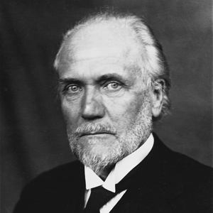
Gustav Cassel
1886-1945
“[M]arginal productivity itself is not an objectively ascertained factor in the pricing problem, but is in fact one of the unknowns in the problem...[A factor's] marginal productivity, then, cannot be defined as anything other than [its] price, for this price represents precisely the contribution of the labour in question to the price of the product. The statement that wages are determined by the marginal productivity of labour thus loses all independent meaning,” (pp.312-313).
Cassel, Gustav, 1918, The Theory of Social Economy
You Can't Easily Measure Marginal Product!
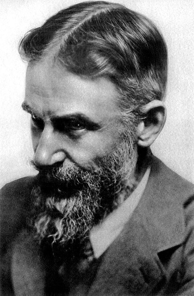
George Bernard Shaw
1856-1950
“[T]hat of giving to every person exactly what he or she has made by his or her labor, seems fair; but when we try to put it into practice we discover, first, that it is quite impossible to find out how much each person has produced,” (p.21).
Shaw, George Bernard, 1928, The Intelligent Woman's Guide to Socialism and Capitalism
You Can't Easily Measure Marginal Product!
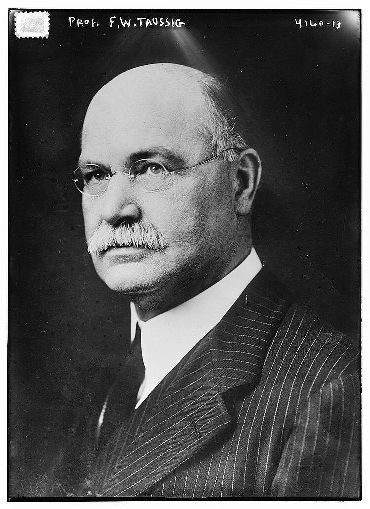
Frank Taussig
1859-1940
“there is no separate product of the tool on the one hand and of the labor using the tool on the other...We can disengage no concretely separable product of labor and capital.”
Taussig, Frank, 1926, Wages and Capital
You Can't Easily Measure Marginal Product!

L: Armen Alchian (1914-2013)
R: Harold Demsetz (1930-2019)
"[A firm] is a team use of inputs and a centralized position of some party in the contractual arrangements of all other inputs. It is the centralized contractual agent in a team productive process," (p.778).
You Can't Easily Measure Marginal Product!

L: Armen Alchian (1914-2013)
R: Harold Demsetz (1930-2019)
"Two men jointly lift heavy cargo into trucks. Solely by observing the total marginal productivity and making pay-weight loaded per day, it is impossible to determine each person's marginal productivity...In team production, marginal products of cooperative team members are not so directly and separably (i.e., cheaply) observable. What a team offers to the market can be taken as the marginal product of the team but not of the team members. The costs of metering or ascertaining the marginal products of the team's members is what calls forth new organizations and procedures," (pp.778).
The Morality of Marginal Productivity
John Bates Clark: The Morality of Marginal Productivity

John Bates Clark
1847—1938
Clark didn't just argue that factors are all paid their marginal products, but that this is a natural law and a moral virtue of markets
- Each factor is paid for its contribution to society
Factor prices (and presumably distribution of income) are not only efficient, they are just
John Bates Clark: The Morality of Marginal Productivity

John Bates Clark
1847—1938
“If each productive function is paid for according to the amount of its product, then each man get what he himself produces. If he works, he gets what he creates by working; if he provides capital, he gets what his capital produces; and if, further, he renders service by coordinating labor and capital, he gets the product that can be separately traced to that function. Only in one of these ways can a man produce anything. If he receives all that he brings into existence through any one of these three functions, he receives all that he creates at all,” (p.7)
Clark, John Bates, 1899, The Distribution of Wealth: A theory of wages, interest and profits
John Bates Clark: The Morality of Marginal Productivity

John Bates Clark
1847—1938
Meant this as a critique of both Karl Marx and Henry George
Georgists believed rent was undeserved, unearned income of landowners: should go to government
Marxists believed profit was exploitative and undeserved (surplus value): belonged to workers
Clark’s Distribution of Wealth argues that marginal productivity theory shows that under competitive markets, each factor is paid its just due
- Labor and land and capital are all necessary for production, and are paid for their productive contributions
John Bates Clark: The Morality of Marginal Productivity

John Bates Clark
1847—1938
Heavily criticized for this normative theory
- Problems: not perfectly competitive, monopolies, labor unions, etc.
- His student, Thorstein Veblen reached the opposite conclusion!
A scarce factor (talent, etc) will command higher prices (and reap economic rents), might be efficient, but is that moral?
Hume’s is-ought gap
More Misconceptions
It sounds like Clark is referring to each individual worker (including the inframarginal workers!) being paid their marginal product
But this is only true for the marginal workers — they “set” the equilibrium wage for all equivalent workers
Recall market supply is the minimum willingness of factor owners to accept, the minimum price necessary to bring a resource to market
Inframarginal workers earn surplus (rents): difference between equilibrium wage and minimum WTA
